How to Make a Thousand Plots Look Good: Data Viz Tips for Parameterized Reporting

Follow Along!

https://rfor.us/cascadia2024

• Who I am
• Who R for the Rest of Us is

• Giving a talk on report design at posit::conf
• If you’re interested in parameterized reporting, chat with Jadey

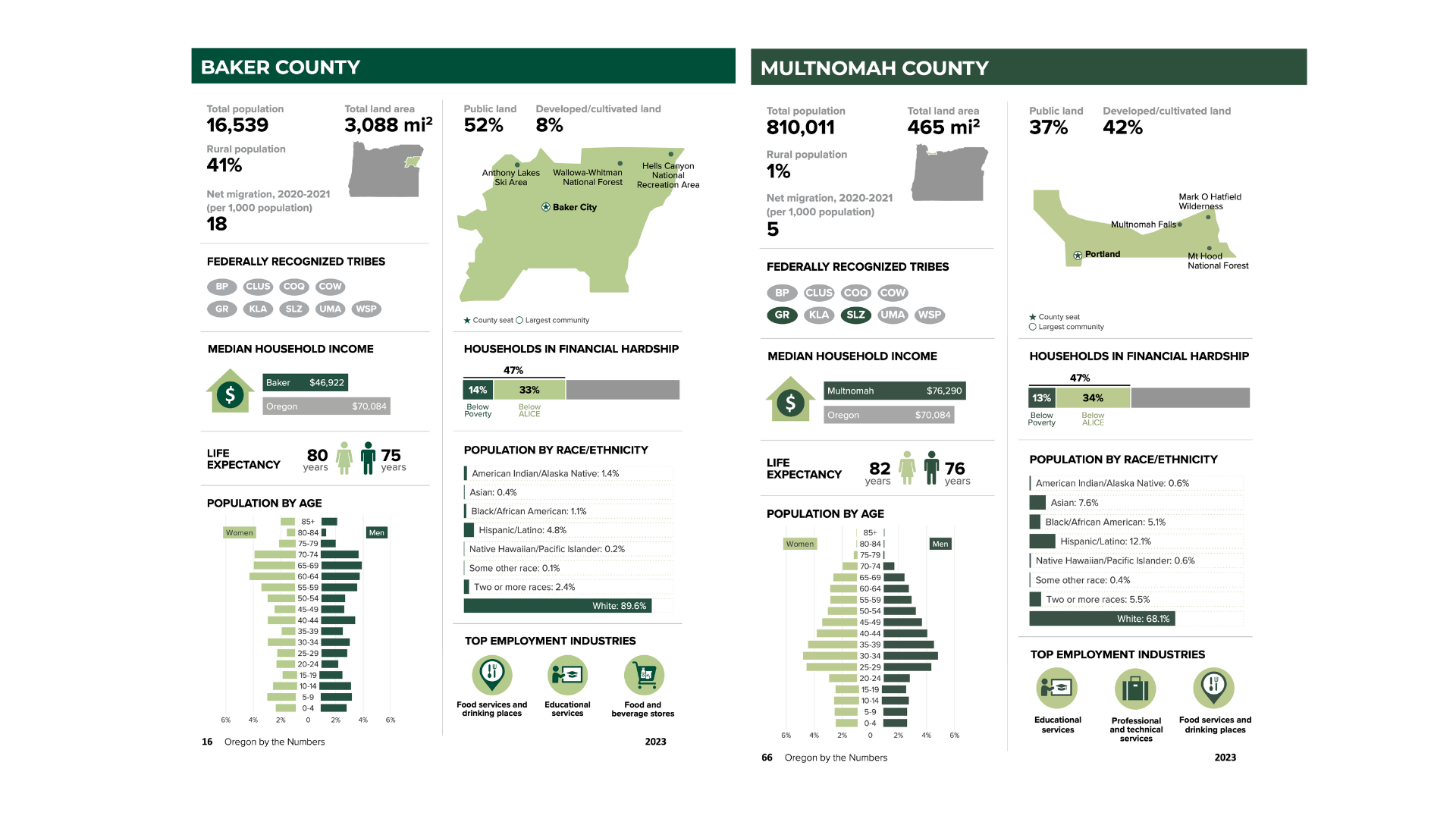
Data Viz Tips for Parameterized Reporting

There is No Magic Package

There are packages to help with all of this, but nothing that can help you avoid thinking deeply about your data

Consider the Outer Limits of Your Data

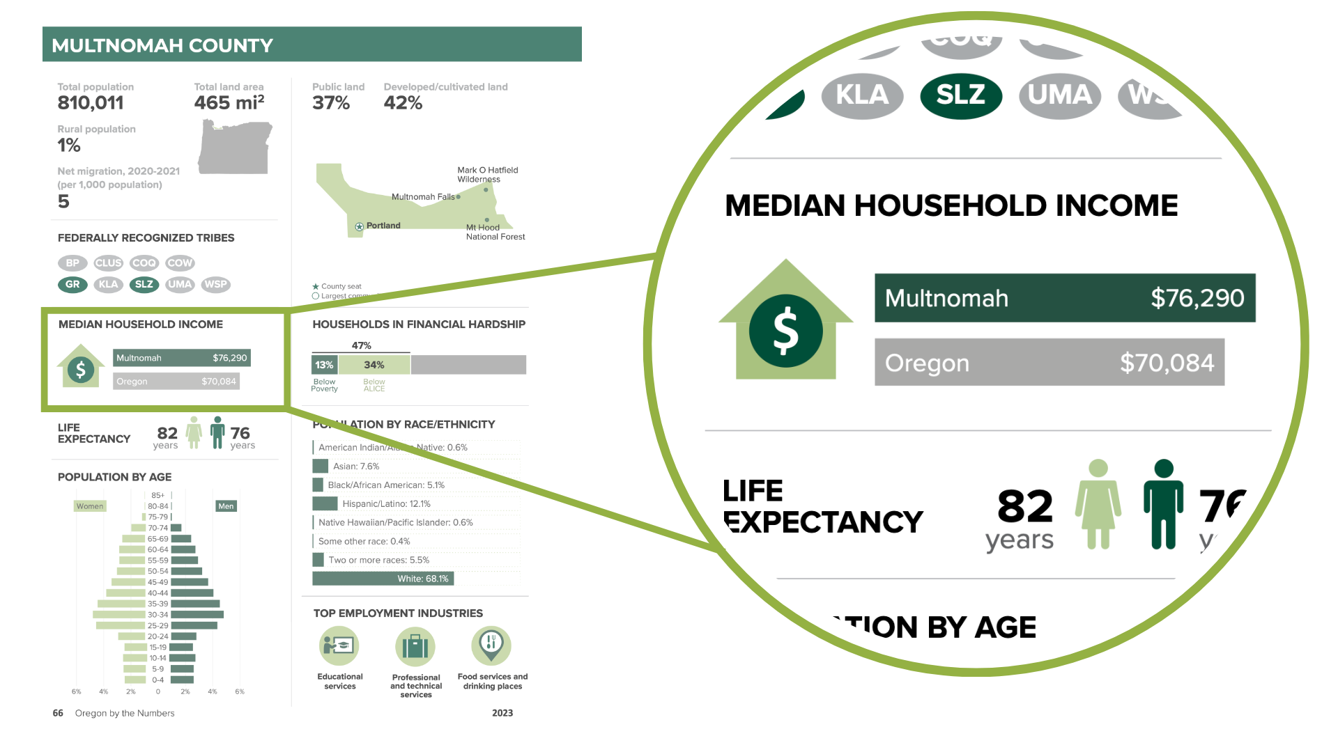
median_income

# A tibble: 37 × 3
   geography amount amount_formatted
   <chr>      <dbl> <chr>           
 1 Oregon     76632 $76,632         
 2 Baker      51657 $51,657         
 3 Benton     72882 $72,882         
 4 Clackamas  95740 $95,740         
 5 Clatsop    68025 $68,025         
 6 Columbia   83265 $83,265         
 7 Coos       57563 $57,563         
 8 Crook      74969 $74,969         
 9 Curry      64300 $64,300         
10 Deschutes  82042 $82,042         
# ℹ 27 more rows

median_income_plot <- function(county_to_plot) {
  median_income |>
    filter(geography %in% c(county_to_plot, "Oregon")) |>
    ggplot(
      aes(
        x = amount,
        y = geography,
        label = amount_formatted,
        fill = geography
      )
    ) +
    geom_col() +
    ...
}

median_income_plot(county_to_plot = "Jackson")

max_median_income <-
  median_income |>
  slice_max(
    order_by = amount,
    n = 1
  ) |>
  pull(amount)

max_median_income

[1] 100121

median_income_plot(county_to_plot = "Jackson") +
  scale_x_continuous(
    limits = c(0, max_median_income)
  )

Minimize Text and Position it Carefully

Text WILL overlap so think proactively about how to avoid it

Don’t Try to Label Everything

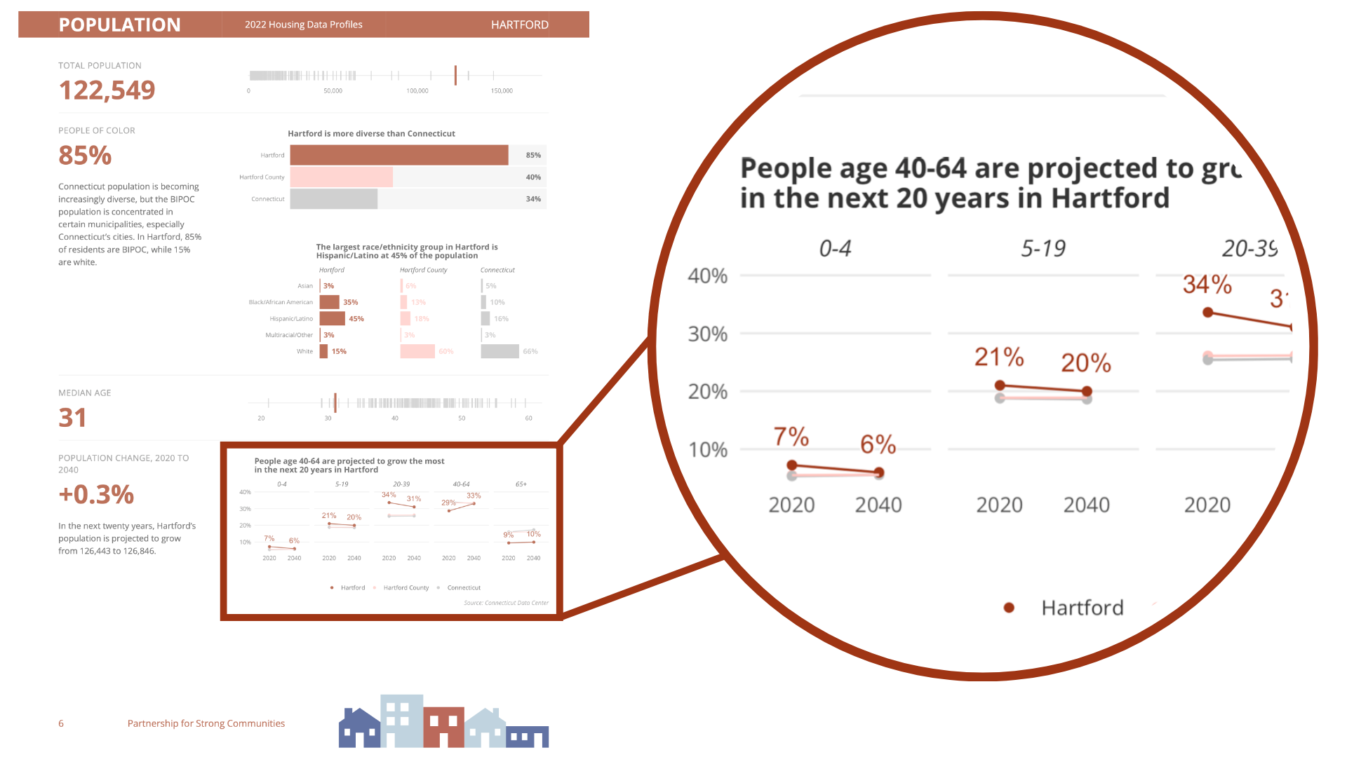
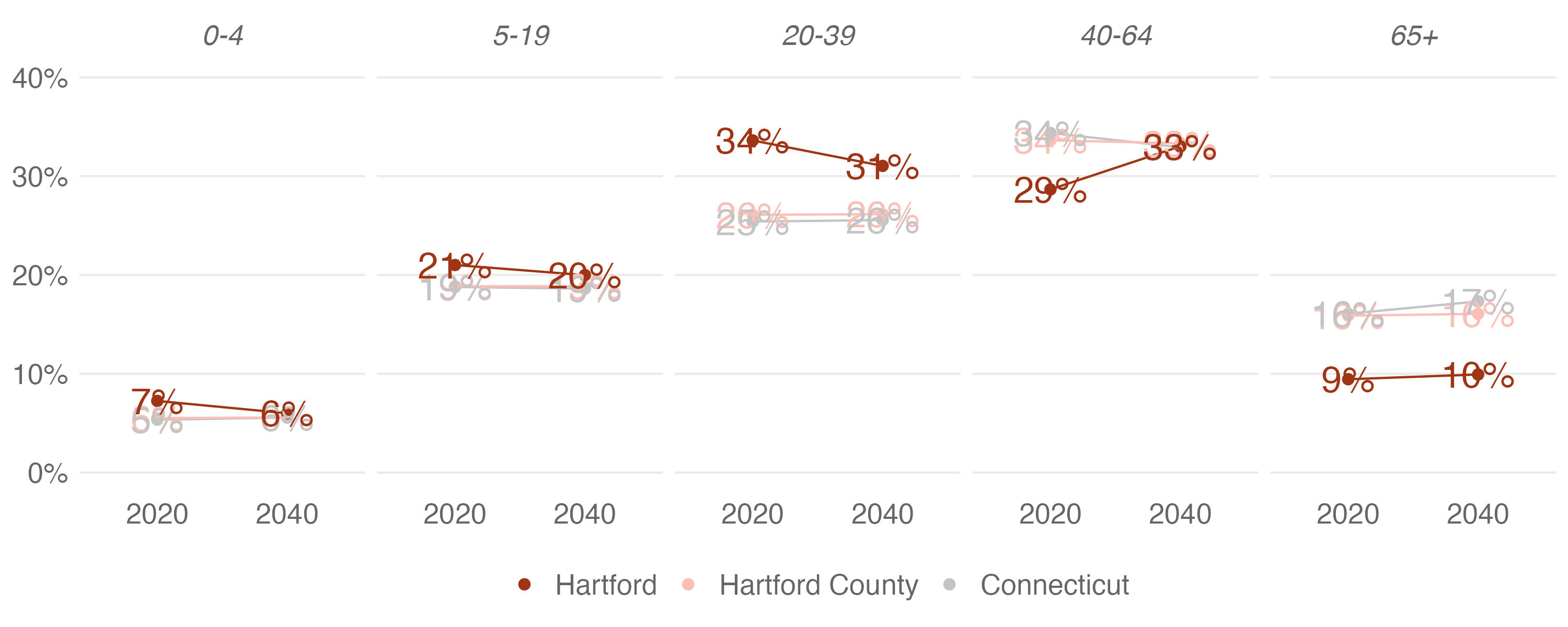
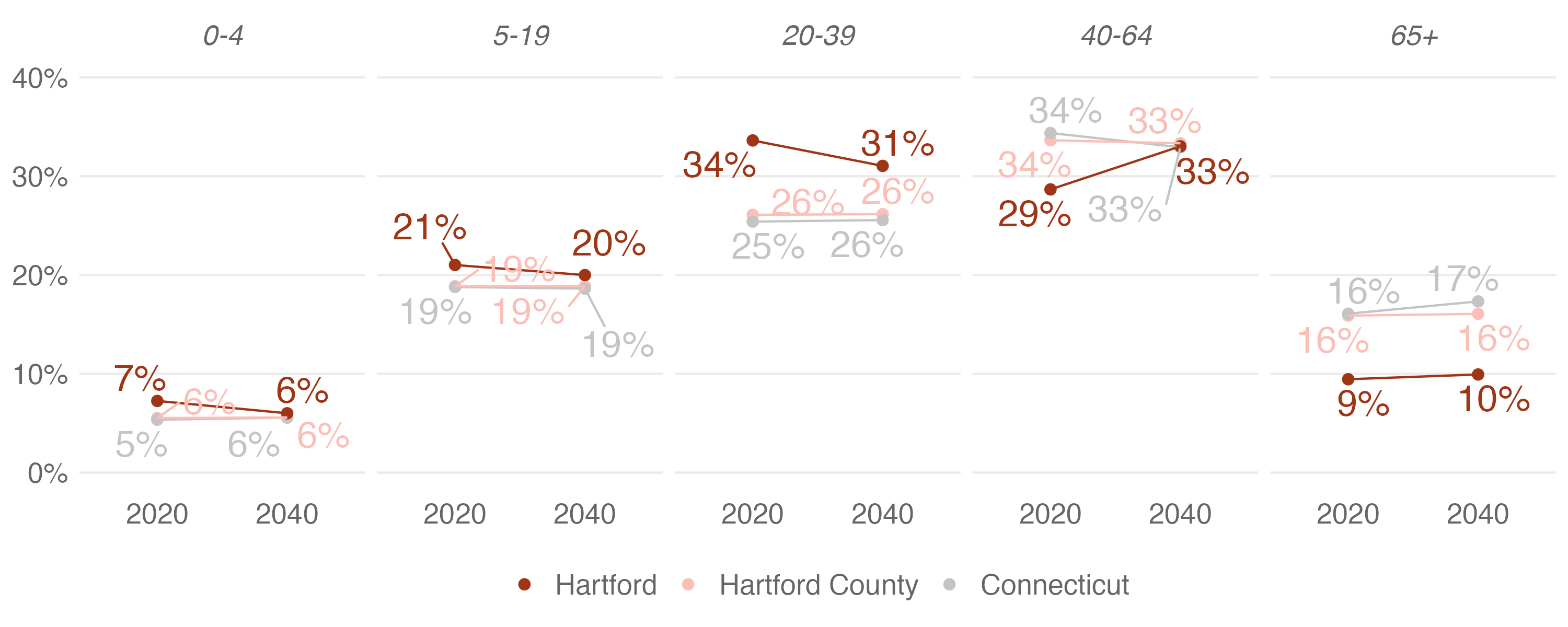
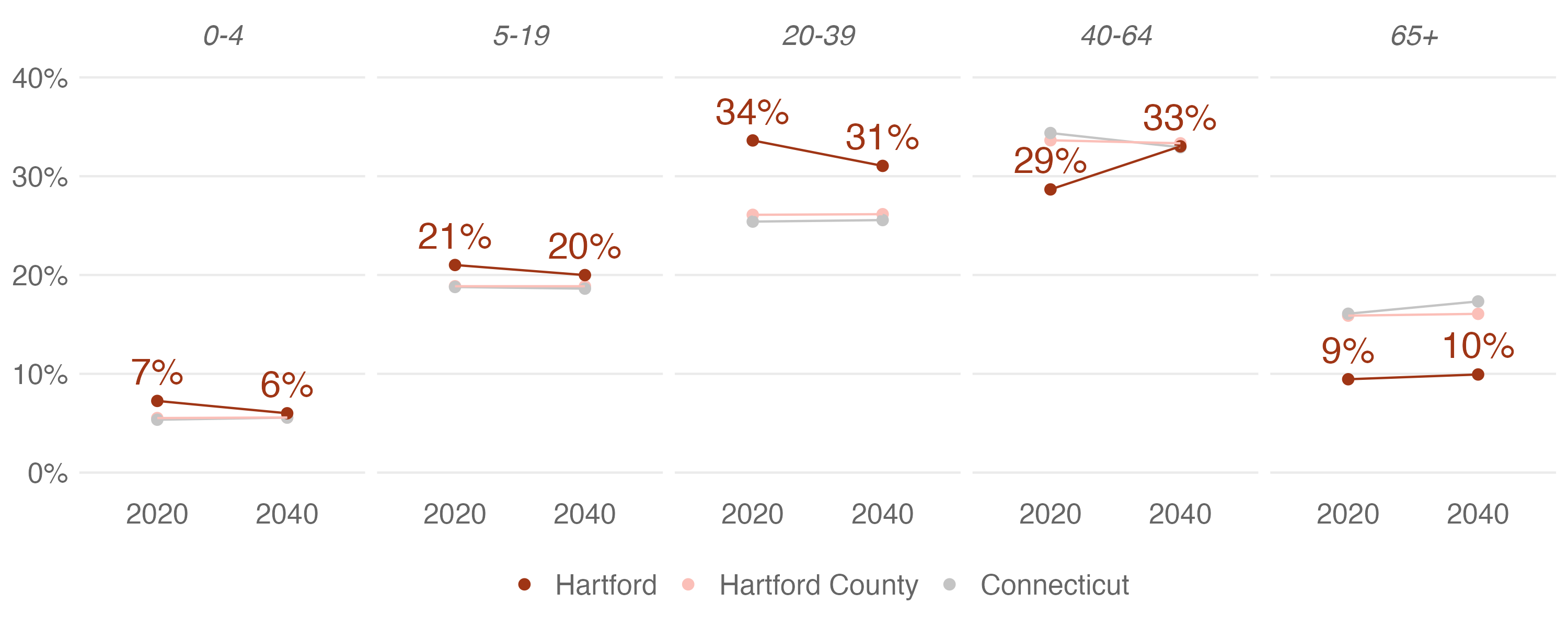
population_projection |>
  filter(location == "Hartford")

# A tibble: 10 × 5
   location year  age_group    pct pct_formatted
   <chr>    <chr> <fct>      <dbl> <chr>        
 1 Hartford 2020  0-4       0.0725 7%           
 2 Hartford 2020  5-19      0.210  21%          
 3 Hartford 2020  20-39     0.336  34%          
 4 Hartford 2020  40-64     0.287  29%          
 5 Hartford 2020  65+       0.0945 9%           
 6 Hartford 2040  0-4       0.0600 6%           
 7 Hartford 2040  5-19      0.200  20%          
 8 Hartford 2040  20-39     0.310  31%          
 9 Hartford 2040  40-64     0.330  33%          
10 Hartford 2040  65+       0.0993 10%          

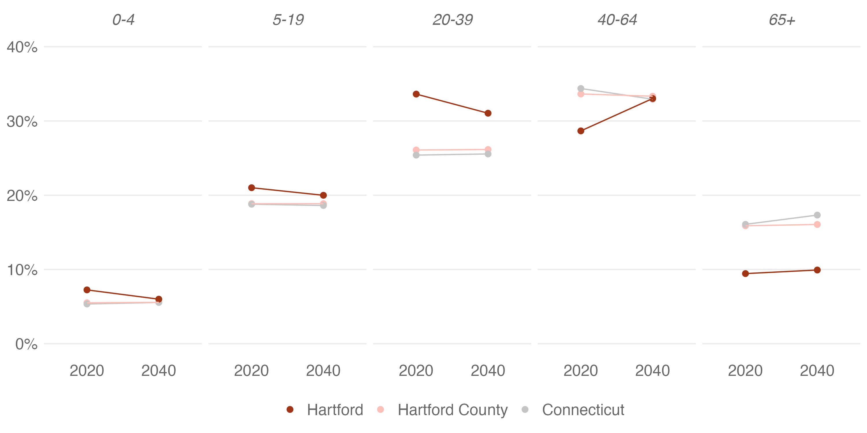
population_projection_plot <- function(town_to_plot, county_to_plot) {
  population_projection |>
    filter(location %in% c(town_to_plot, county_to_plot, "Connecticut")) |>
    ggplot(aes(
      x = year,
      y = pct,
      color = location,
      group = location
    )) +
    geom_point() +
    geom_line() +
    ...
}

population_projection_plot(
  town_to_plot = "Hartford",
  county_to_plot = "Hartford County"
)

population_projection_plot(
  town_to_plot = "Hartford",
  county_to_plot = "Hartford County"
) +
  geom_text(
    aes(
      label = pct_formatted
    )
  )

library(ggrepel)

population_projection_plot(
  town_to_plot = "Hartford",
  county_to_plot = "Hartford County"
) +
  geom_text_repel(
    aes(
      label = pct_formatted
    )
  )

population_projection_plot(
  town_to_plot = "Hartford",
  county_to_plot = "Hartford County"
) +
  geom_text(
    data = population_projection |> filter(location == "Hartford"),
    nudge_y = 0.03,
    aes(
      label = pct_formatted
    )
  )

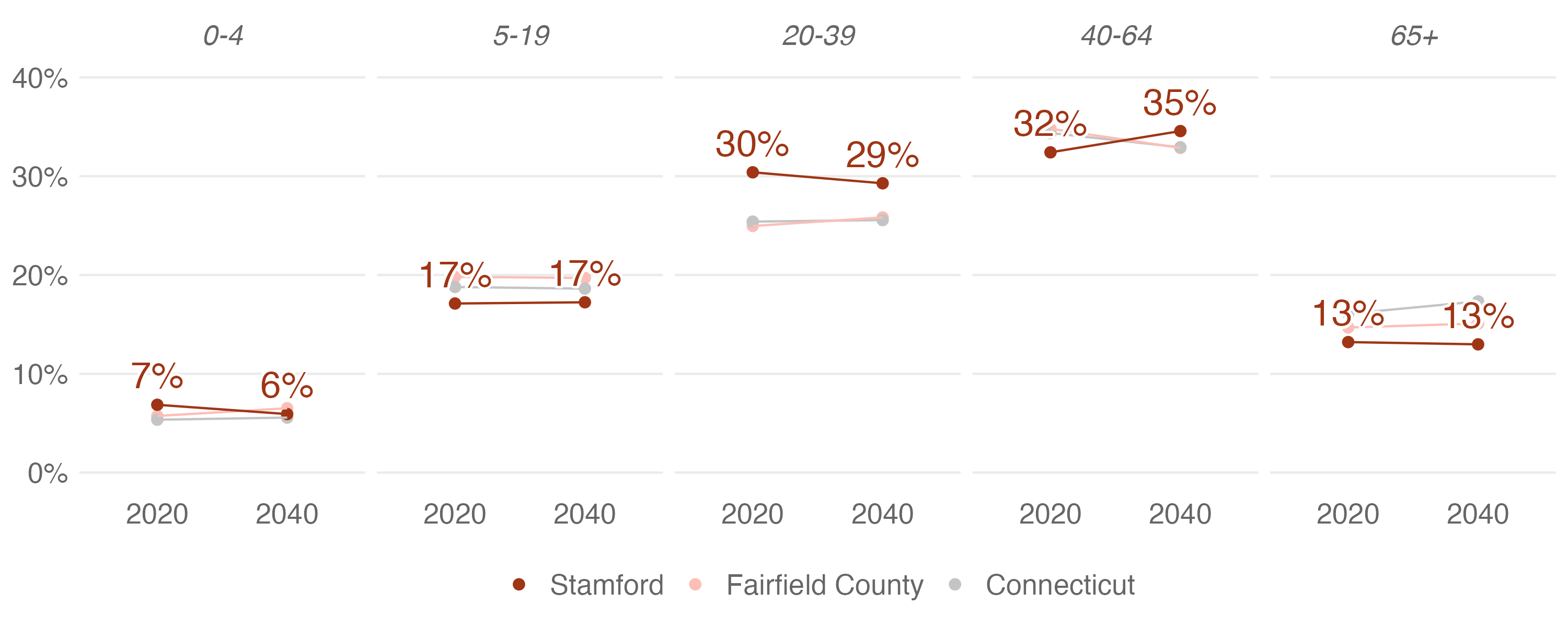
population_projection_plot(
  town_to_plot = "Stamford",
  county_to_plot = "Fairfield County"
) +
  geom_text(
    data = population_projection |> filter(location == "Stamford"),
    nudge_y = 0.03,
    aes(
      label = pct_formatted
    )
  )

library(shadowtext)

population_projection_plot(
  town_to_plot = "Stamford",
  county_to_plot = "Fairfield County"
) +
  geom_shadowtext(
    data = population_projection |> filter(location == "Stamford"),
    bg.color = "white",
    nudge_y = 0.03,
    aes(
      label = pct_formatted
    )
  )

Hide Small Values

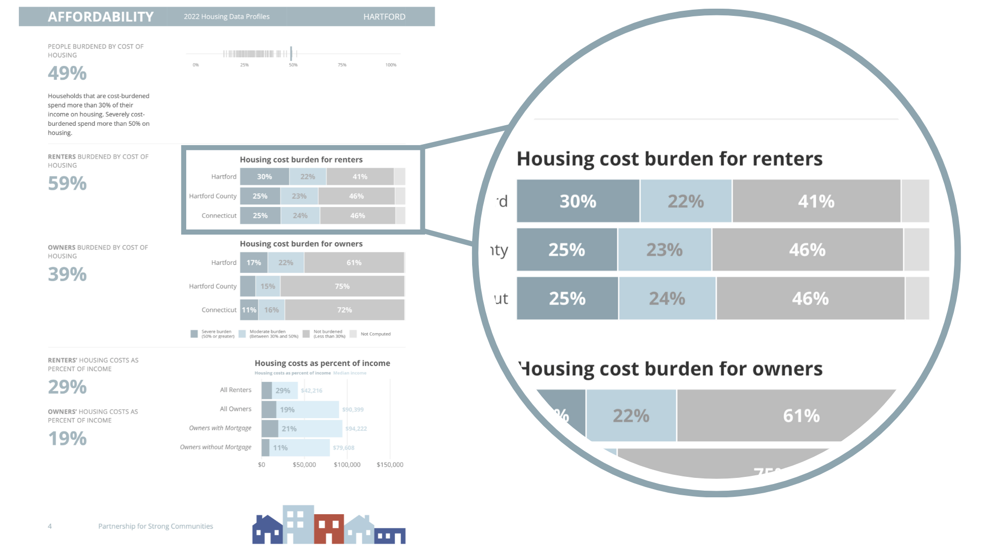
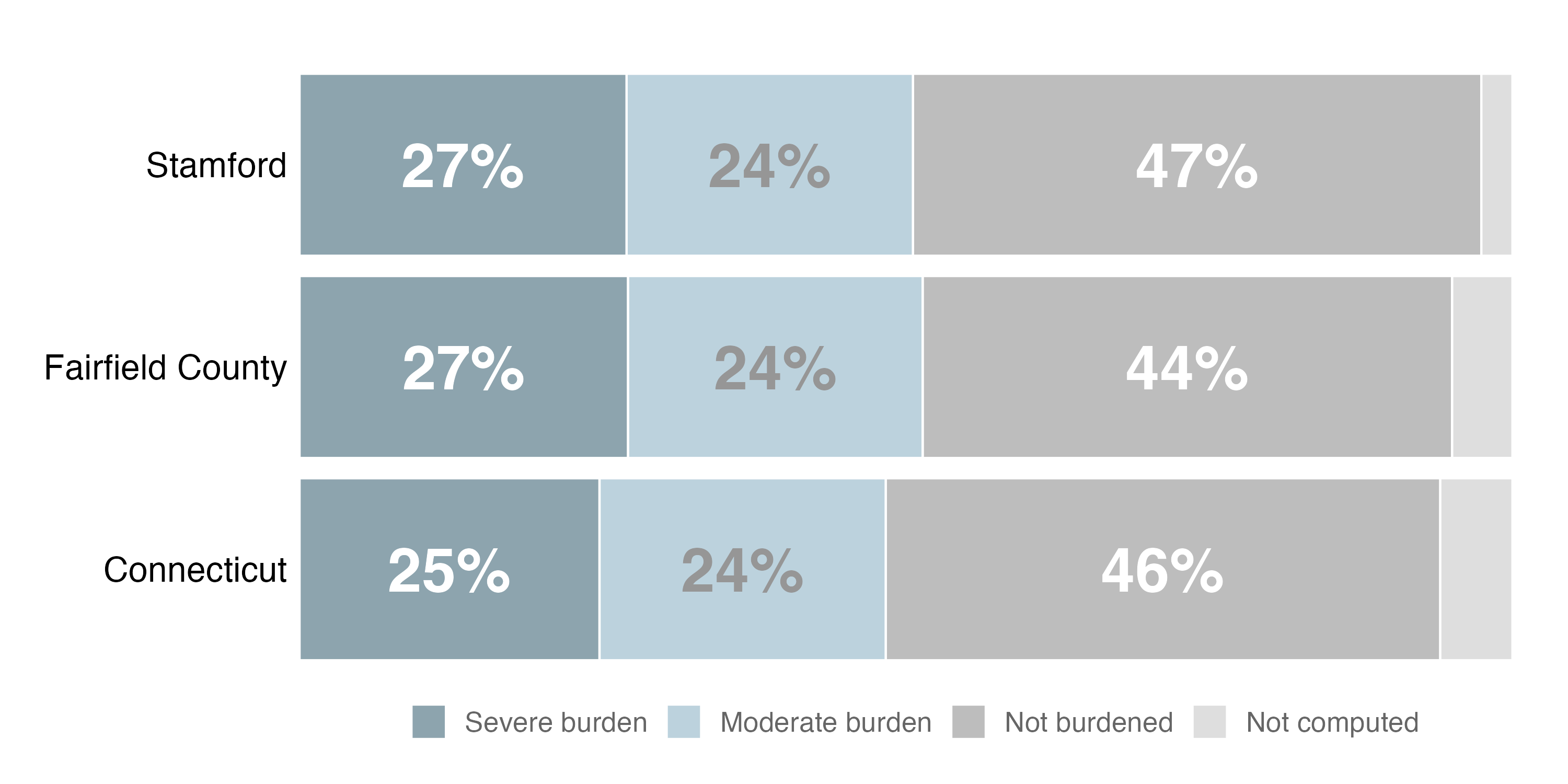
housing_cost_burden 

# A tibble: 694 × 4
   location   burden_level       pct pct_formatted
   <fct>      <fct>            <dbl> <chr>        
 1 Bethel     Not burdened    0.381  38%          
 2 Bethel     Moderate burden 0.352  35%          
 3 Bethel     Severe burden   0.229  23%          
 4 Bethel     Not computed    0.0385 4%           
 5 Bridgeport Not burdened    0.358  36%          
 6 Bridgeport Moderate burden 0.260  26%          
 7 Bridgeport Severe burden   0.332  33%          
 8 Bridgeport Not computed    0.0494 5%           
 9 Brookfield Not burdened    0.501  50%          
10 Brookfield Moderate burden 0.228  23%          
# ℹ 684 more rows

housing_cost_burden_plot <- function(town_to_plot, county_to_plot) {
  housing_cost_burden |>
    filter(location %in% c(town_to_plot, county_to_plot, "Connecticut")) |>
    ggplot(aes(
      x = pct,
      y = location,
      fill = burden_level,
      label = pct_formatted
    )) +
    geom_col() +
    geom_text(position = position_stack(vjust = 0.5)) +
    ...
}

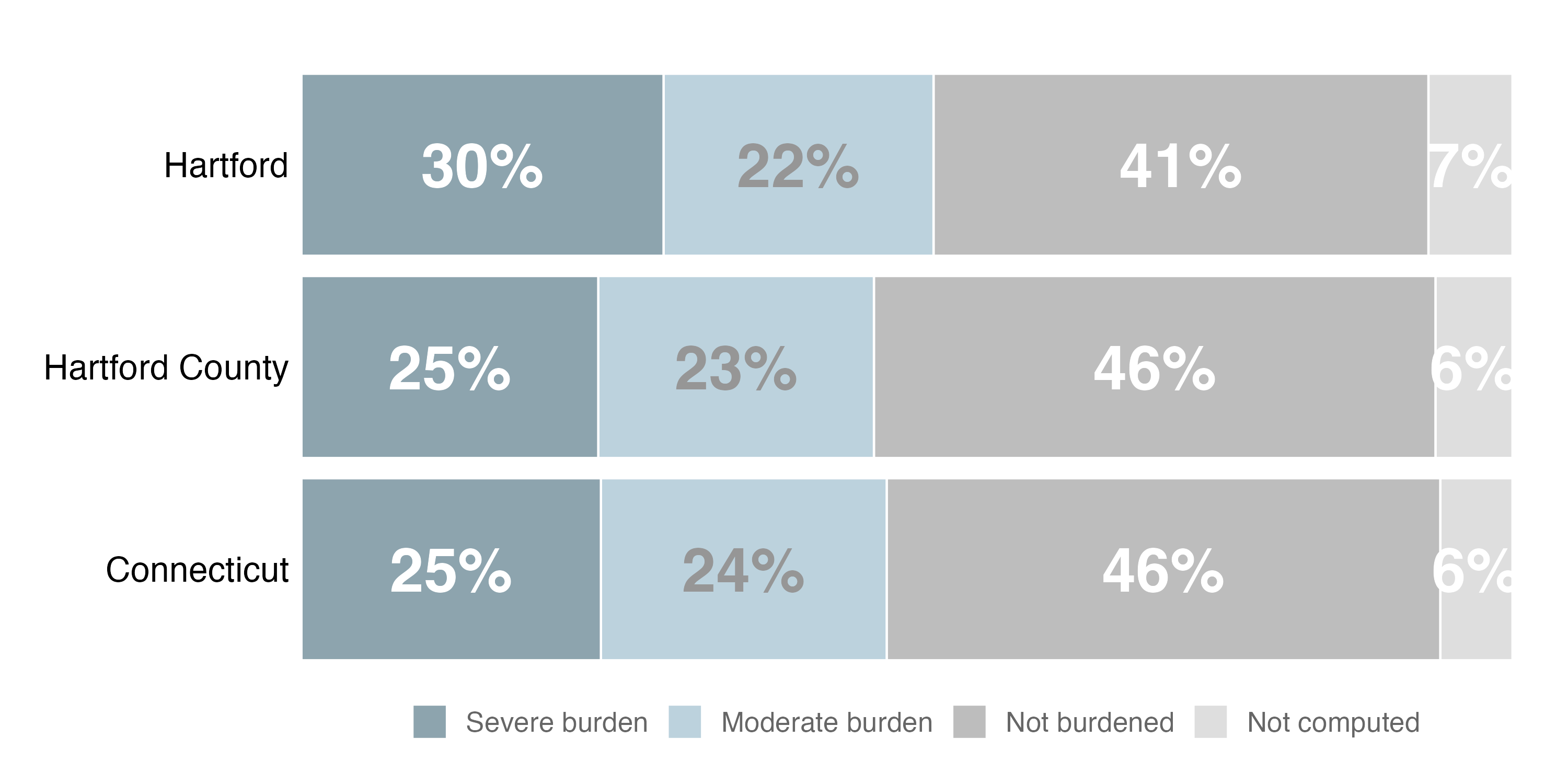
housing_cost_burden_plot(
  town_to_plot = "Hartford",
  county_to_plot = "Hartford County"
)

housing_cost_burden |> 
  filter(location == "Hartford")

# A tibble: 4 × 4
  location burden_level       pct pct_formatted
  <fct>    <fct>            <dbl> <chr>        
1 Hartford Not burdened    0.409  41%          
2 Hartford Moderate burden 0.223  22%          
3 Hartford Severe burden   0.299  30%          
4 Hartford Not computed    0.0694 7%           

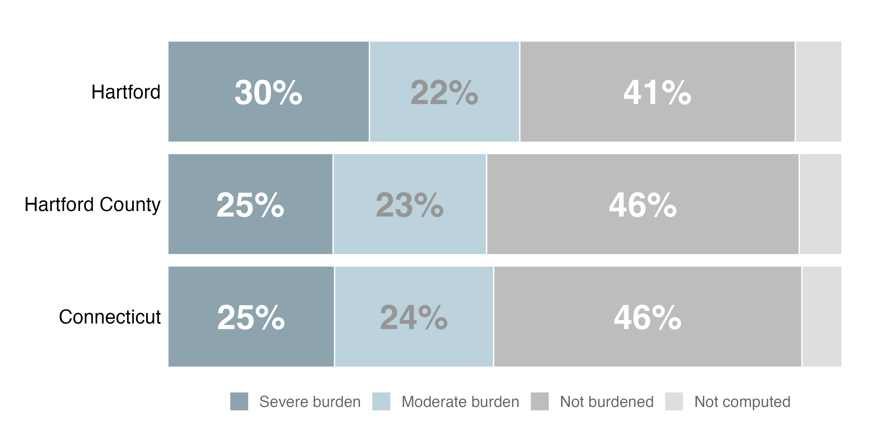
housing_cost_burden <-
  housing_cost_burden |>
  mutate(pct_formatted = if_else(pct > 0.07, pct_formatted, NA))

housing_cost_burden |>
  filter(location == "Hartford")

# A tibble: 4 × 4
  location burden_level       pct pct_formatted
  <fct>    <fct>            <dbl> <chr>        
1 Hartford Not burdened    0.409  41%          
2 Hartford Moderate burden 0.223  22%          
3 Hartford Severe burden   0.299  30%          
4 Hartford Not computed    0.0694 <NA>         

housing_cost_burden_plot(
  town_to_plot = "Hartford",
  county_to_plot = "Hartford County"
)

housing_cost_burden_plot(
  town_to_plot = "Stamford",
  county_to_plot = "Fairfield County"
)

Don’t Put Text Where it Could Be Obscured

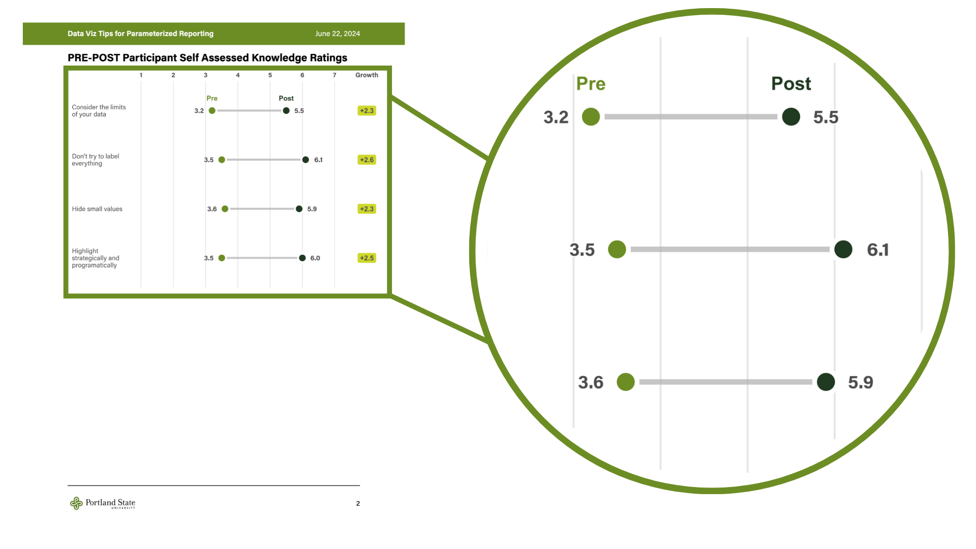
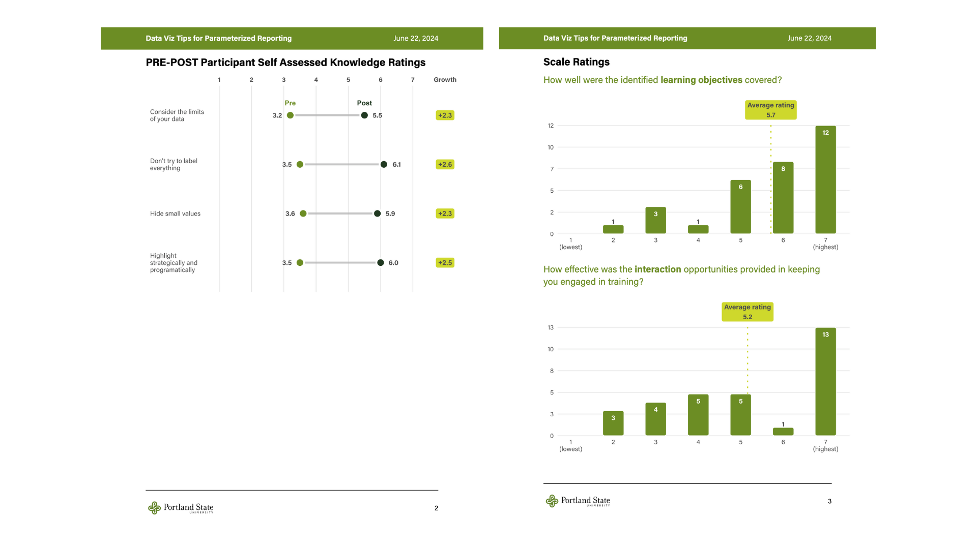
pre_post_data

# A tibble: 2 × 6
  question   timing rating growth growth_formatted growth_text_position
  <chr>      <chr>   <dbl>  <dbl> <glue>                          <dbl>
1 Question 1 Pre       1.6   NA   <NA>                             NA  
2 Question 1 Post      4.2    2.6 +2.6                              2.9

pre_post_plot <- function(df) {
  df |>
    ggplot(aes(
      x = rating,
      y = question,
      fill = timing
    )) +
    geom_line() +
    geom_point(shape = 21) +
    ...
}

pre_post_data |>
  pre_post_plot()

pre_post_data |>
  pre_post_plot() +
  # Ratings within points
  geom_text(
    aes(label = rating),
    color = "white"
  ) +
  # Pre/post labels
  geom_text(
    aes(
      label = timing,
      color = timing
    )
  ) +
  # Growth label
  geom_text(
    aes(
      x = growth_text_position,
      label = growth_formatted
    )
  )

pre_post_data

# A tibble: 2 × 6
  question   timing rating growth growth_formatted growth_text_position
  <chr>      <chr>   <dbl>  <dbl> <glue>                          <dbl>
1 Question 2 Pre       3.5 NA     <NA>                            NA   
2 Question 2 Post      3.6  0.100 +0.1                             3.55

pre_post_data <-
  pre_post_data |>
  mutate(rating_text_position = case_when(
    timing == "Pre" ~ rating - 0.2,
    timing == "Post" ~ rating + 0.2
  ))

pre_post_data |>
  select(question, timing, rating, rating_text_position)

# A tibble: 2 × 4
  question   timing rating rating_text_position
  <chr>      <chr>   <dbl>                <dbl>
1 Question 2 Pre       3.5                  3.3
2 Question 2 Post      3.6                  3.8

pre_post_data |>
  pre_post_plot() +
  geom_text(
    aes(
      x = rating_text_position,
      label = rating
    )
  ) +
  geom_text(
    aes(
      x = rating_text_position,
      label = timing
    )
  ) +
  ...

pre_post_data |>
  pre_post_plot() +
  geom_text(
    aes(
      x = rating_text_position,
      label = rating
    )
  ) +
  geom_text(
    aes(
      x = rating_text_position,
      label = timing
    )
  ) +
  ...

pre_post_data |>
  pre_post_plot() +
  geom_label(
    aes(
      x = 6,
      label = growth_formatted
    )
  ) +
  ...

Highlight Strategically and Programatically

Use a range of aesthetic properties

Color

Size

Shadow

Outline

Opacity

Color

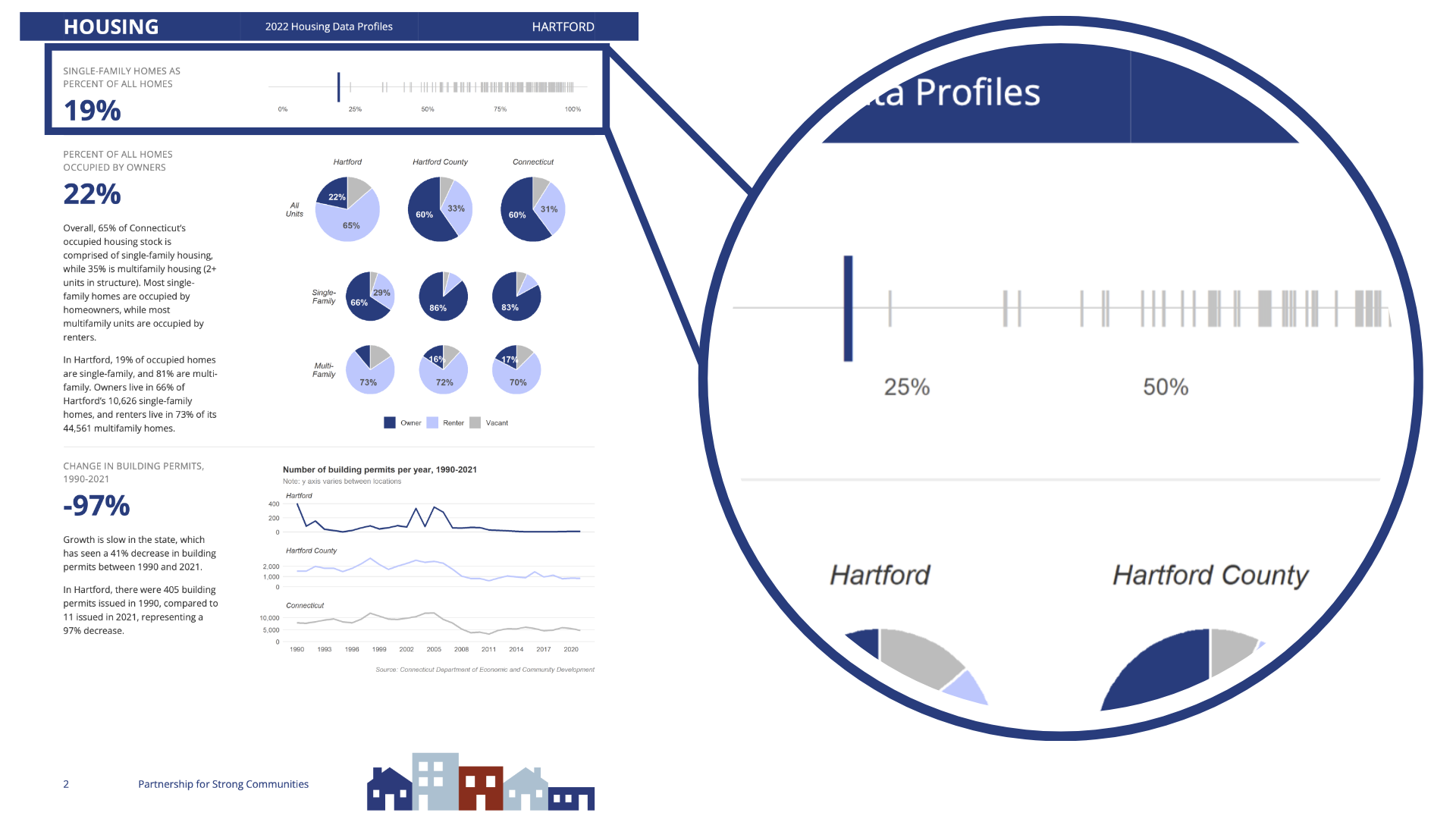
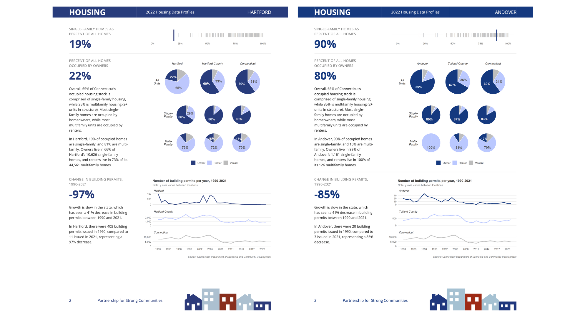
single_family_homes

# A tibble: 169 × 2
   location       pct
   <fct>        <dbl>
 1 Andover      0.897
 2 Ansonia      0.548
 3 Ashford      0.850
 4 Avon         0.844
 5 Barkhamsted  0.956
 6 Beacon Falls 0.717
 7 Berlin       0.807
 8 Bethany      0.958
 9 Bethel       0.746
10 Bethlehem    0.944
# ℹ 159 more rows

single_family_homes_plot <- function() {
  single_family_homes |>
    ggplot(
      aes(
        x = pct,
        y = 1
      )
    ) +
    geom_point(
      shape = 124,
      color = "grey80"
    ) +
    ...
}

single_family_homes_plot()

single_family_homes_plot() +
  geom_point(
    data = single_family_homes |> filter(location == "Hartford"),
    shape = 124,
    color = "#15397f"
  )

Talk about how I’m adding layers on top of other layers here

Size

single_family_homes_plot() +
  geom_point(
    data = single_family_homes |> filter(location == "Hartford"),
    shape = 124,
    color = "#15397f",
    size = 15
  )

single_family_homes_plot() +
  geom_point(
    data = single_family_homes |> filter(location == "Stamford"),
    shape = 124,
    color = "#15397f",
    size = 15
  )

Shadow

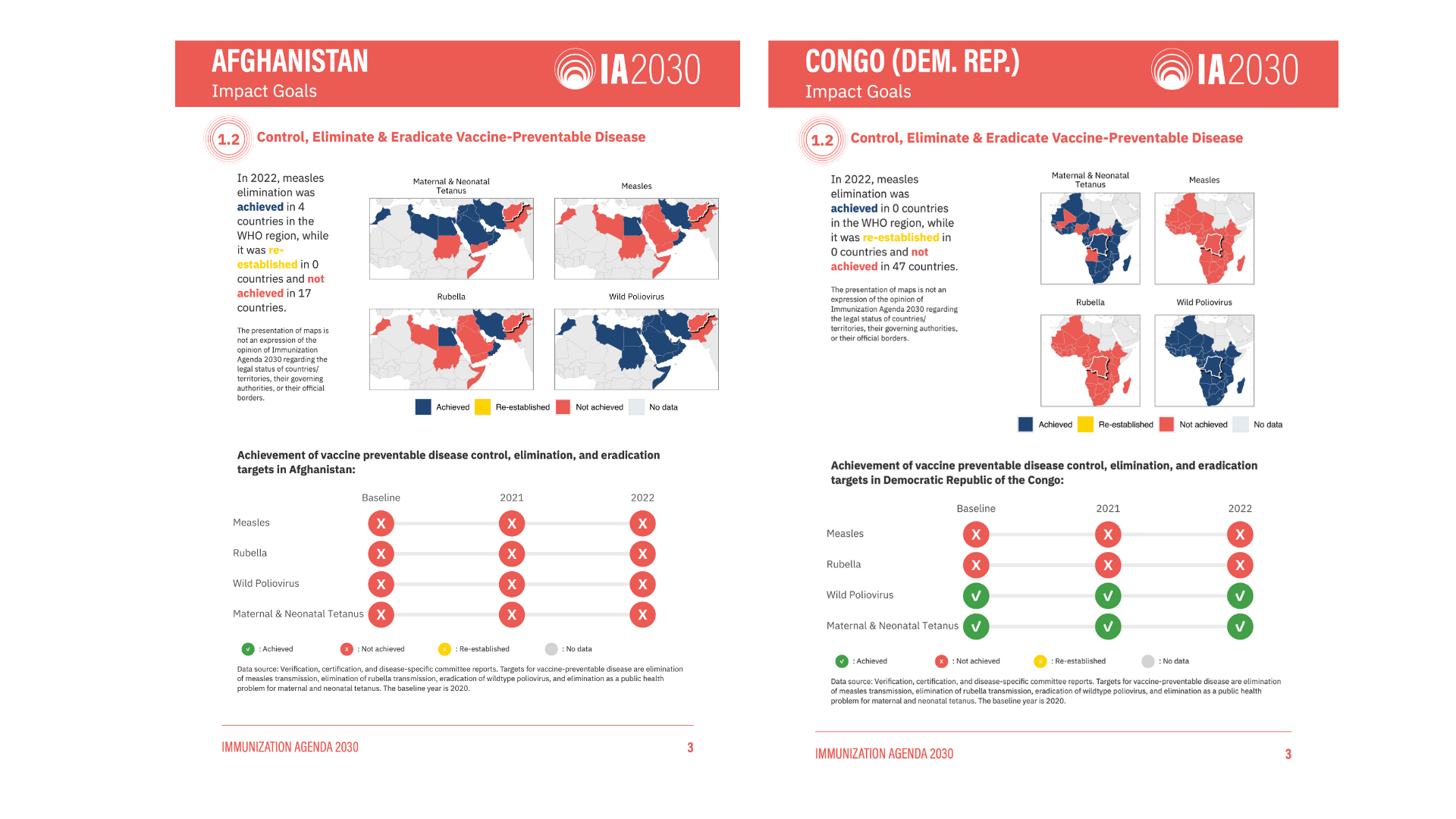
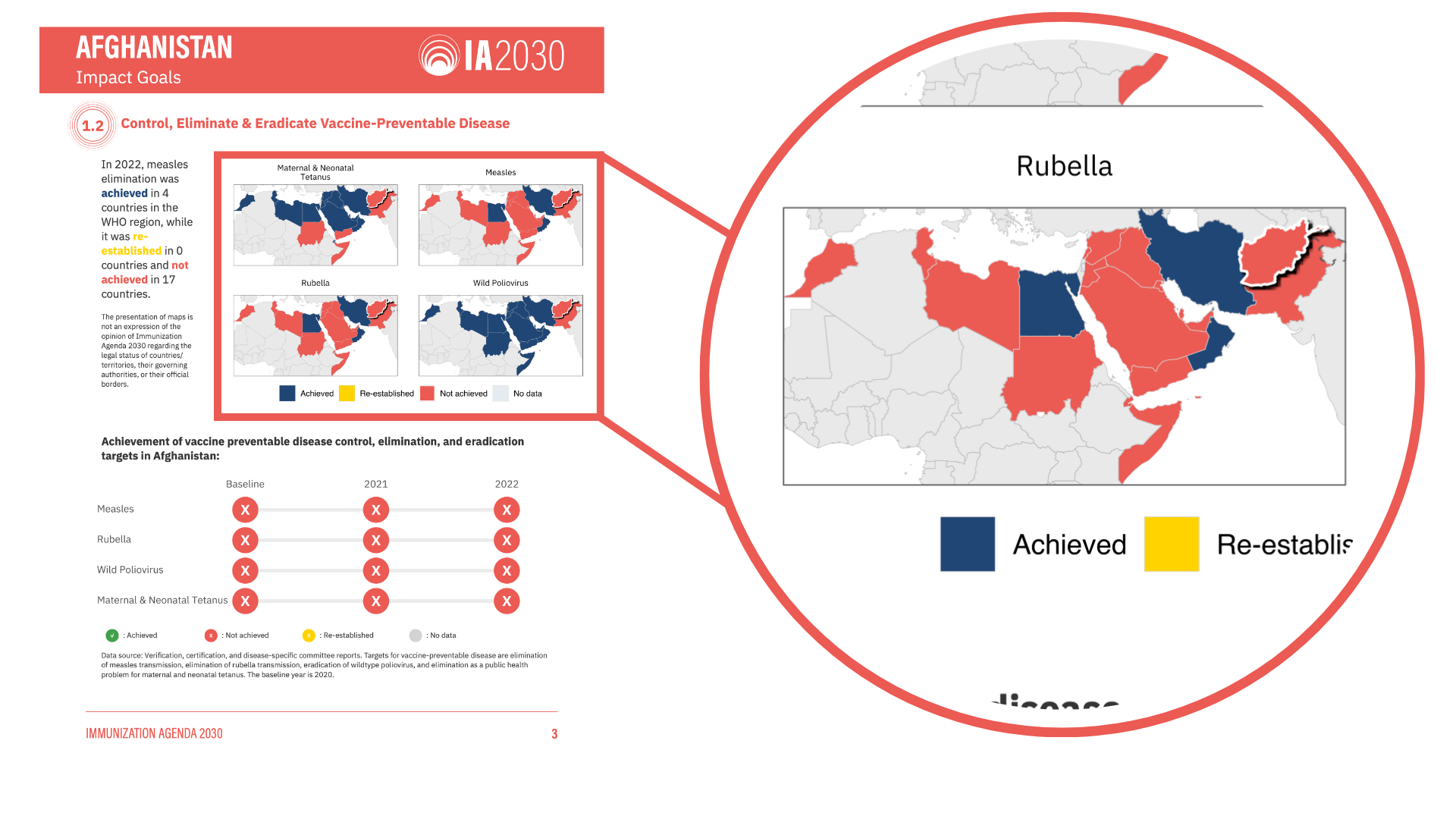
rubella

Simple feature collection with 69 features and 3 fields
Geometry type: MULTIPOLYGON
Dimension:     XY
Bounding box:  xmin: -1466635 ymin: -185219 xmax: 8649202 ymax: 4806756
Projected CRS: WGS 84 / World Mercator
First 10 features:
                    country region       status                       geometry
1               Afghanistan      1 Not achieved MULTIPOLYGON (((8328599 444...
2      United Arab Emirates      1 Not achieved MULTIPOLYGON (((6004988 275...
3                     Benin      0 Not achieved MULTIPOLYGON (((392437.9 12...
4              Burkina Faso      0 Not achieved MULTIPOLYGON (((21538.26 16...
5                   Bahrain      1     Achieved MULTIPOLYGON (((5634224 299...
6  Central African Republic      0 Not achieved MULTIPOLYGON (((2701448 953...
7                     China      0 Not achieved MULTIPOLYGON (((8649200 420...
8                  Cameroon      0 Not achieved MULTIPOLYGON (((1719405 819...
9                  Djibouti      1 Not achieved MULTIPOLYGON (((4780514 122...
10                  Algeria      0 Not achieved MULTIPOLYGON (((961591.4 43...

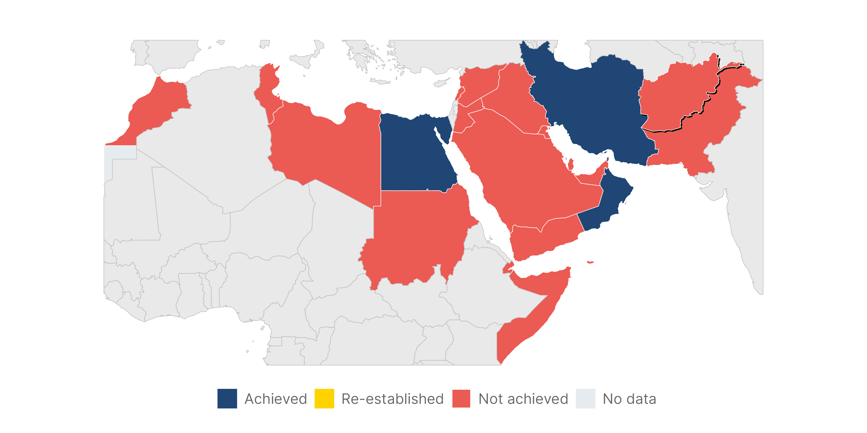
region_map <- function() {
  ggplot() +
    geom_sf(
      data = rubella |> filter(region == 1),
      aes(fill = status)
    ) +
    geom_sf(
      data = rubella |> filter(region == 0),
      fill = "lightgrey",
      alpha = 0.5
    ) +
    ...
}

region_map()

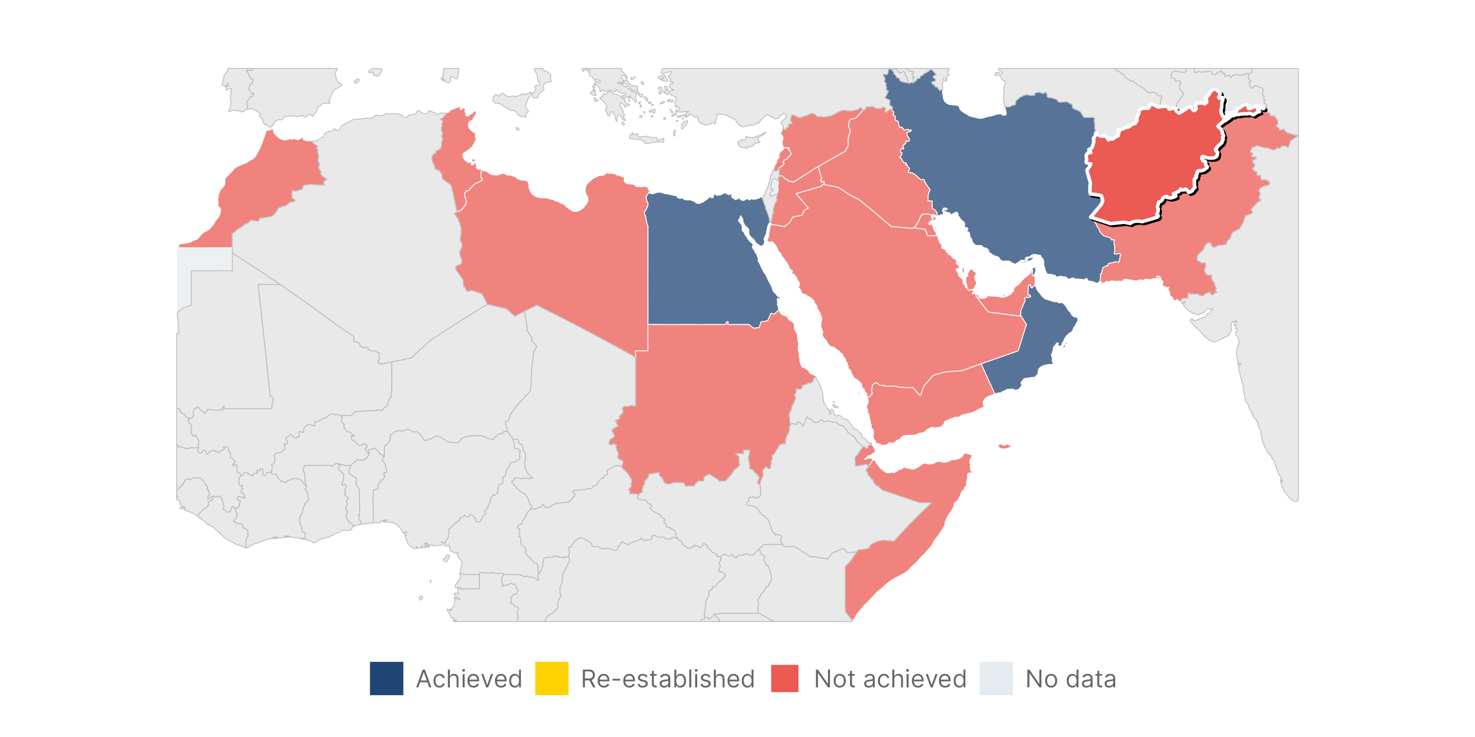
library(ggfx)

region_map() +
  with_shadow(
    geom_sf(
      data = rubella |> filter(country == "Afghanistan")
    ),
    ...
  )

Outline

region_map() +
  with_shadow(
    geom_sf(
      data = rubella |> filter(country == "Afghanistan")
    ),
    linewidth = 0.8,
    color = "white",
    ...
  )

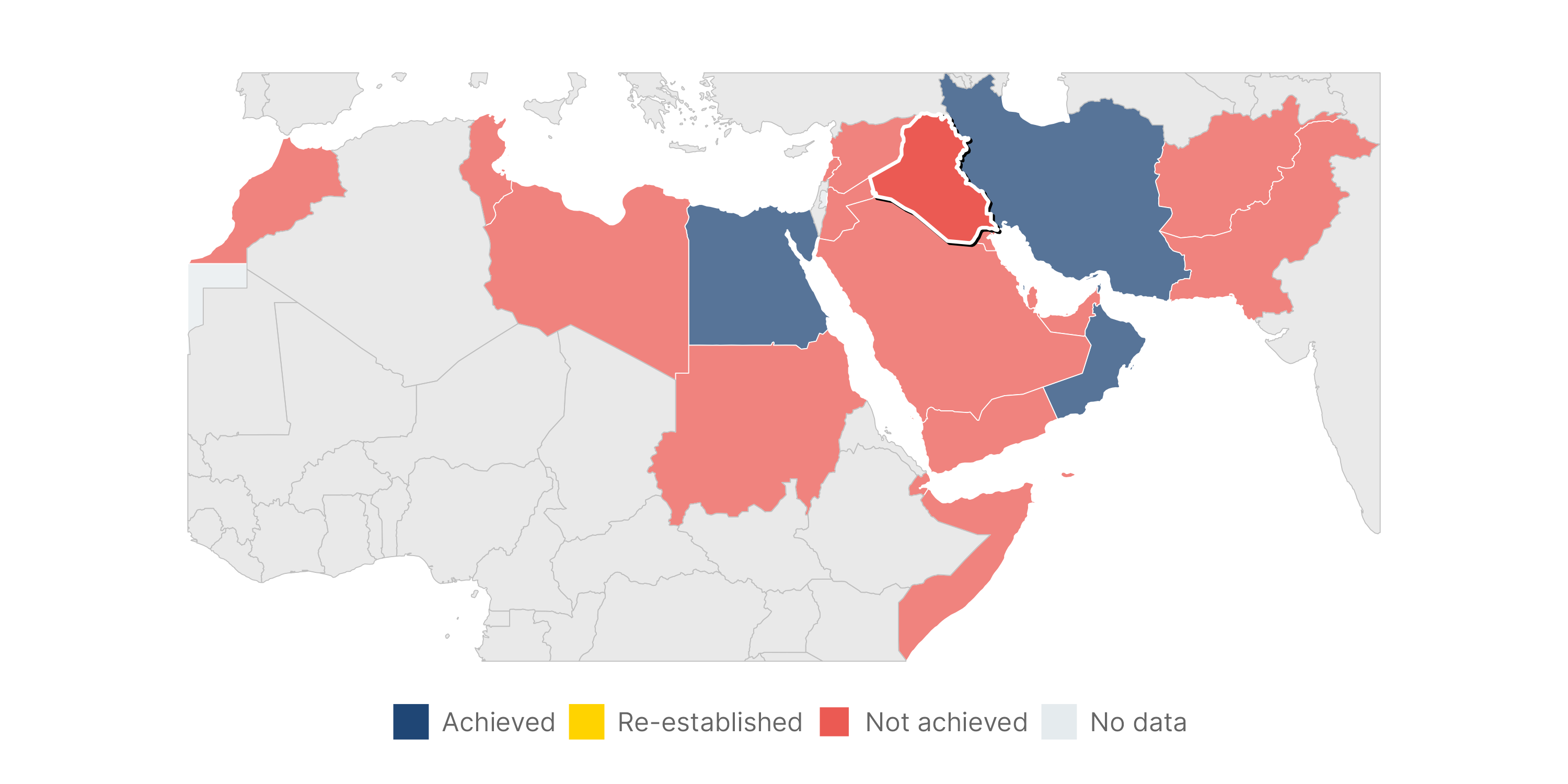
Opacity

region_map <- function() {
  ggplot() +
    geom_sf(
      data = rubella |> filter(region == 1),
      aes(fill = status),
      alpha = 0.75
    ) +
    geom_sf(
      data = rubella |> filter(region == 0),
      fill = "lightgrey",
      alpha = 0.5
    ) +
    ...
}

region_map() +
  with_shadow(
    geom_sf(
      data = rubella |> filter(country == "Afghanistan")
    ),
    linewidth = 0.8,
    color = "white",
    ...
  )

region_map() +
  with_shadow(
    geom_sf(
      data = rubella |> filter(country == "Iraq")
    ),
    linewidth = 0.8,
    color = "white",
    ...
  )

Conclusion

1. Consider the outer limits of your data

2. Minimize text and position it carefully

3. Highlight strategically and programatically with a range of aesthetic properties

4. Packages are helpers, but you are the one who has to do the thinking